The Retirement Calculator From Hell - Part II

One of the joys of this Web site is the appreciation I get for dispensing investment commentary. And by far, the piece that has elicited the greatest response is "The Retirement Calculator From Hell."

Long story short: Almost all retirement calculations are done with a straightforward amortization algorithm (via a handheld financial calculator or a software product) that does not take into account the fluctuation in returns. The risk being, if you get a string of bad years at the front end of your retirement, you could run out of money long before the calculated number of years based on an overall rate of return.

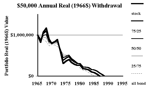
For example, the real return on an 80/20 mix of large- and small-cap stocks for the 30-year period 1966-1995 was 5.9%. Plugging this return into a financial calculator tells us that an annual real withdrawal (of the beginning principal, inflation-adjusted) of 7.2% over this 30-year period is possible. Yet the following two plots tell a more worrisome story: Even a real 5% withdrawal rate leads to an Alpo diet long before 30 years is up. Paradoxically, in this scenario, because bonds offset poor stock returns in the first years, adding intermediate treasuries, with only a 2.9% real return for the period, helps stretch the money. These portfolios were rebalanced annually. (Readers of the original piece may notice that this is even grimmer than the plots first published. Thanks to reader Bob Beeman for catching a computational error in the first article. The corrected graphs now appear in both articles.) I apologize for the messy plots: all five of the portfolios, from all-stock to all-bond, decay at nearly the same rate, and it is difficult to visually separate them out.

Even this may be an overly rosy scenario. With the S&P yielding just 1.2% in dividends, a 5.9% real return requires either an inflation-adjusted earnings/dividend growth rate of 4.7% or a further expansion of multiples. Neither of these are events I’d want to bet my golden years on.

So we have a real problem. First, standard amortization doesn’t factor in return variability. Second, historical data do not take into account the reduced equity risk premium we currently expect.

Is there a better way? Yes. I have received quite a few e-mails from engineering types about Monte Carlo analysis, and I’ve always been dubious about using it for portfolio optimization. As a simple retirement calculator, however, Monte Carlo simulation offers clear-cut advantages over running raw historical data or simple amortization algorithms.

What exactly is Monte Carlo, and how do we deploy it for retirement planning? First, a few assumptions... Let’s say that we’re examining a 100% stock portfolio for which we’ve assumed a 7% real return, with a returns standard deviation of 12%. Because of "variance drag" (more on this four paragraphs below), in order to obtain an annualized return of 7.0%, we need an average annual return of 7.7%. (If you are confused about the difference between average and annualized returns, take a look at the discussion of this about a third of the way into Chapter 1 of The Intelligent Asset Allocator.) Let’s further assume that we’re withdrawing 5% of our initial capital in real dollars each year.

Monte Carlo simulates returns variability by adding in a random component to each period’s return. Say we’ve decided to look at a 50-year period and are examining annual returns. That’s 50 time periods. In each, we generate a random number with a normal distribution. This means that two-thirds of these random numbers will be between –1.0 and +1.0, 95% will lie between –2.0 and +2.0, and nearly 99.9% will be between –3.0 and +3.0. Let’s say that the random number that pops up for the first year is –1.15. The return for the first period would then be:

7.7% - (1.15 x 12%) = -6.1%

Remember too, in each period we have to withdraw 5% of the initial capital. We generate 50 different random normal numbers to calculate a run of 50 years. The run is categorized as a "success" if we have any money left after 50 years, and a "failure" if we don’t. Repeating the process thousands of times gives a fairly solid statistical estimation of the true success rate.

Monte Carlo simulation requires a large amount of computation. For example, 100,000 runs of 50-year simulations using monthly returns involves 60,000,000 separate monthly calculations. As a practical matter, this is beyond the memory capacity of most desktop spreadsheet systems. (The outer limits of microprocessor/spreadsheet analysis is about 30 annual periods x 10,000 runs.)

There are also some computational nuances to consider. The most important one is this: varying SD also varies return, via so-called "variance drag." Say you begin with an annual return of 10% each and every year (zero SD). You will of course wind up with a 10% annualized return over the long haul. But crank in a normally-distributed random term with 20% SD, and you find that your range of annualized returns falls to a median of about 8%. This needs to be adjusted for, as it was in the above example when the assumed 7% annualized return was replaced by an equivalent average annual return of 7.7%. Changing annual returns and SDs to monthly ones raises other computational issues.

So there’s no getting around a dedicated application for this purpose. My colleague David Wilkinson graciously cooperated with a nifty bit of code that clips along at about 4,000 runs per second of 600 months each on my first-generation Pentium system.

(For those who want to explore the spreadsheet option, I have posted a 100-run by 30-year sample here.)

The first table below shows the results for monthly returns and withdrawals for an "old-paradigm" returns scenario, with high (7%) real stock returns, low (2.5%) real bond returns. I assumed a relatively low stock SD of 12%. This is worth a comment here. When one runs Monte Carlo simulations of stock returns using the historical 15%-20% SD, one comes up with higher long-period (>20 years) variability than is actually observed. The reason is, over the long haul stock returns have a tendency to mean-revert. To correct for this, I’ve lowered the SD a bit.

Next, I added bonds to the mix, assuming a 2.5% real return and an SD of 5% for intermediate-term instruments. A zero stock-bond correlation was assumed. The rebalanced overall portfolio real return/SD data were computed using another of David Wilkinson’s programs, MvoPlus. The return and SD data are displayed in the first two columns. These were then fed into David’s new MCRetire program, generating the first table. The 30-year success rates for withdrawals of 4%, 5%, 6%, and 7% of the the initial principal amount in real terms are listed in the last four columns.

30-Year Success Rates (Monthly Withdrawals)
Returns: Stocks 7%, Bonds 2.5%

	Return	SD	4.0%	5.0%	6.0%	7.0%
Stocks	7.0%	12.0%	98.7%	93.4%	81.0%	63.3%
75/25	6.0%	9.09%	99.3%	93.4%	76.0%	50.3%
50/50	4.9%	6.5%	99.6%	91.4%	61.2%	24.9%
25/75	3.8%	4.8%	99.3%	77.4%	24.8%	2.6%
Bonds	2.5%	5.0%	87.2%	33.4%	3.7%	1.3%

I also examined a "new-paradigm" returns scenario with 4.5%/3.5% stock/bond returns in the second table.

30-Year Success Rates (Monthly Withdrawals)
Returns: Stocks 4.5%, Bonds 3.5%

	Return	SD	4.0%	5.0%	6.0%	7.0%
Stocks	4.5%	12.0%	88.8%	70.4%	48.0%	28.3%
75/25	4.4%	9.09%	94.3%	75.2%	46.6%	22.2%
50/50	4.2%	6.5%	98.2%	80.1%	41.3%	12.0%
25/75	3.9%	4.8%	99.5%	81.1%	28.9%	3.4%
Bonds	3.5%	5.0%	98.2%	68.3%	18.5%	0.2%

Obviously, the new paradigm with its low equity risk premium is less forgiving than the old paradigm. You can safely withdraw about 5% of initial principal under the old paradigm, but only about 4% under the new. No surprise here. And it’s also no surprise that under the new paradigm, very high levels (75%) of bonds seem to be optimal. But even under the old paradigm at the safe 4% and 5% withdrawal rates, a 25% bond contribution is well-tolerated. Finally, if your withdrawal rate is "too high" for safety, 100% stocks give you your best (albeit poor) chance of success under both scenarios.

A few philosophical observations are in order. One of finance's ironies is that concentrating your portfolio is the best way to become very rich; it is also the best way to become poor. So an investor's first duty is to decide which of these two goals is paramount. This article is aimed at those who seek safety in retirement, not great riches. (If you haven't saved enough to sustain your chosen retirement lifestyle, then in fact you do maxmize your chances of success by investing aggressively, as can be seen in the last column of the second table. But this is damage control—you are simply optimizing grim odds.)

Obviously, Monte Carlo has its flaws. But playing with your portfolio's return/risk assumptions gives you a good idea of the tradeoffs between these inputs and retirement success. And it’s lot more realistic than using a simple amortization calculation... by a country mile.

For those of you who are interested, David’s MCRetire is currently in beta testing and should be available soon. The estimated price is in the $20-$30 range. If you want details about David's software products, you can get them at Efficient Solutions.

Copyright © 2001, William J. Bernstein